Stream processing in Python with Redpanda and Quix
Build an app in three steps using the simplest tech in streaming data
Author: Merlin Carter
A few years ago, the Redpanda blog featured a post on how to build a stream processing application with Redpanda and Faust. Since then, the Python stream processing ecosystem has matured, and more options are now available to Python developers — such as Bytewax and Quix.
So, it’s time to revisit that tutorial and try some steps with one of these newer players. This post will focus on Quix, which lets developers use the entire Python ecosystem to build stream processing pipelines in fewer lines of code.
In this post, you’ll learn how to build a stream processing application by integrating the Quix Streams Python library with Redpanda. You’ll also get some background on why Python libraries like Faust, Bytewax, and Quix have emerged to compete with existing Java-centric options.
What is Quix?
Quix is a complete platform for developing, deploying, and monitoring stream processing pipelines. It provides an innovative stream processing framework through its open-source library and cloud platform, designed for teams looking to build real-time data pipelines using Python and DataFrames (a tabular representation of streaming data). Here, I’ll focus on the open-source Python library: Quix Streams.
In a sense, Quix Streams is very similar to Faust. It has been described as “…more or less Faust 2.0 — pure Python with the annoying bits handled.”
Before you install Quix Streams, set up a virtual environment that uses Python version 3.8 or higher.
Once you have activated your virtual environment, install the Quix Streams library with the following command:
pip install quixstreams
What you’ll build
Like the Faust version of this post, you’ll build an application that calculates the rolling aggregations of temperature readings from various sensors. The temperature readings will come in at a relatively high frequency, and this application will aggregate the readings and output them at a lower time resolution (every 10 seconds).
This application includes code that generates synthetic sensor data, but in a real-world scenario, this data could come from many kinds of sensors, such as sensors installed in a fleet of vehicles or a warehouse full of machines.
Here’s an illustration of the basic architecture:
All the code used in this demo is available in this GitHub repository. But before we dive into the tutorial, let’s break down the diagram so you know what’s what.
Components of a stream processing pipeline
The previous diagram reflects the main components of a stream processing pipeline: The sensors are the data producers, Redpanda is the streaming data platform, and Quix is the stream processor.
Data producers
These are bits of code attached to systems that generate data, such as firmware on ECUs (Engine Control Units), monitoring modules for cloud platforms, or web servers that log user activity. They take that raw data and send it to the streaming data platform in a format that that platform can understand.
Streaming data platform
This is where you put your streaming data. It plays more or less the same role as a database does for static data. But instead of tables, you use topics. Otherwise, it has similar features to a static database. You’ll want to manage who can consume and produce data, and what schemas the data should adhere to.
Unlike a database though, the data is constantly in flux, so it’s not designed to be queried. You’d usually use a stream processor to transform the data and put it elsewhere for data scientists to explore or sink the raw data into a queryable system optimized for streaming data, such as RisingWave or Apache Pinot.
However, this isn’t an ideal solution for automated systems that are triggered by patterns in streaming data (such as recommendation engines). In this case, you definitely want to use a dedicated stream processor.
Stream processors
These application components perform continuous operations on the data as it arrives. They could be compared to just regular old microservices that process data in any application back end, but there’s one big difference. For microservices, data arrives in drips like droplets of rain, and each “drip” is processed discreetly.
For a stream processor, the data arrives as a continuous gush of water. A filtration system would be quickly overwhelmed unless you change the design. I.e., break the stream up and route smaller streams to a battery of filtration systems.
That’s how stream processors work. They’re designed to be horizontally scaled and work in parallel as batteries. And they never stop. They process the data continuously, outputting the filtered data to the streaming data platform, which acts as a reservoir for streaming data.
To complicate things, stream processors often need to keep track of data received previously, as in the windowing example you’ll try out here.
Note that there are also “data consumers” and “data sinks” — systems that consume the processed data (such as front end applications and mobile apps) or store it for offline analysis (data warehouses like Snowflake or AWS Redshift). Since we won’t cover those in this tutorial, I’ll skip them now.
Tutorial: aggregating sensor readings in a blink
1. Set up the streaming data platform
In this tutorial, you’ll use Redpanda as your streaming data platform (of course!). It’s simply the easiest and most performant option.
To get started, you’ll need a Redpanda cluster. The easiest way to get one is to follow the Redpanda Self-hosted Quickstart. This guide shows you how to use Docker Compose to quickly spin up a cluster, including the Redpanda Console.
Alternatively, you can sign up for a free trial with Redpanda Serverless. Just note down your bootstrap server address which you’ll need later in the tutorial.
2. Create the streaming applications
Create separate files to produce and process your streaming data. This makes it easier to manage the running processes independently. Here’s an overview of the two files that you’ll create:
- The stream producer:
sensor_stream_producer.py
Generates synthetic temperature data and produces (i.e., writes) that data to a “raw data” source topic in Redpanda. It produces the data at a resolution of approximately 20 readings every 5 seconds, or around 4 readings a second.
- The stream processor:
sensor_stream_processor.py
Consumes (reads) the raw temperature data from the “source” topic, and performs a tumbling window calculation to decrease the resolution of the data. It calculates the average of the data received in 10-second windows so you get a reading for every 10 seconds. It then produces these aggregated readings to the agg-temperatures topic in Redpanda.
The stream processor does most of the heavy lifting and is the core of this tutorial. The stream producer is a stand-in for a proper data ingestion process. For example, in a production scenario, you might use something like the Quix MQTT connector to get data from your sensors and produce it to a topic.
For a tutorial, it’s simpler to simulate the data, so let’s get that set up first.
2a. Creating the stream producer
Start by creating a new file called sensor_stream_producer.py and define the main Quix application. (This example has been developed on Python 3.10, but different versions of Python 3 should work as well, as long as you can run pip install quixstreams.)
Create the file sensor_stream_producer.py and add all the required dependencies (including Quix Streams)
from dataclasses import dataclass, asdict # used to define the data schema
from datetime import datetime # used to manage timestamps
from time import sleep  # used to slow down the data generator
import uuid # used for message id creation
import json # used for serializing data

from quixstreams import Application
Then, define a Quix application and destination topic to send the data.
app = Application(broker_address='localhost:19092')

destination_topic = app.topic(name='raw-temp-data', value_serializer="json")
The value_serializer parameter defines the format of the expected source data (to be serialized into bytes). In this case, you’ll be sending JSON.
Let’s use the dataclass module to define a basic schema for the temperature data and add a function to serialize it to JSON.
@dataclass
class Temperature:
    ts: datetime
    value: int

    def to_json(self):
        # Convert the dataclass to a dictionary
        data = asdict(self)
        # Format the datetime object as a string
        data['ts'] = self.ts.isoformat()
        # Serialize the dictionary to a JSON string
        return json.dumps(data)
Next, add the code that sends the mock temperature sensor data into our Redpanda source topic.
i = 0
with app.get_producer() as producer:
    while i < 10000:
        sensor_id = random.choice(["Sensor1", "Sensor2", "Sensor3", "Sensor4", "Sensor5"])
       temperature = Temperature(datetime.now(), random.randint(0, 100))
        value = temperature.to_json()

        print(f"Producing value {value}")
        serialized = destination_topic.serialize(
            key=sensor_id, value=value, headers={"uuid": str(uuid.uuid4())}
        )
        producer.produce(
            topic=destination_topic.name,
            headers=serialized.headers,
            key=serialized.key,
            value=serialized.value,
        )
        i += 1
        sleep(random.randint(0, 1000) / 1000)
This generates 1000 records separated by random time intervals between 0 and 1 second. It also randomly selects a sensor name from a list of 5 options.
Now, try out the producer by running the following in the command line:
python sensor_stream_producer.py
You should see data being logged to the console like this:
[data produced]
Once you’ve confirmed that it works, stop the process for now (you’ll run it alongside the stream processing process later).
2b. Creating the stream processor
The stream processor performs three main tasks: 1) consume the raw temperature readings from the source topic, 2) continuously aggregate the data, and 3) produce the aggregated results to a sink topic.
Let’s add the code for each of these tasks. In your IDE, create a new file called sensor_stream_processor.py.
First, add the dependencies as before:
import os
import random
import json
from datetime import datetime, timedelta
from dataclasses import dataclass
import logging
from quixstreams import Application


logging.basicConfig(level=logging.INFO)
logger = logging.getLogger(__name__)
Let’s also set some variables that our stream processing application needs:
TOPIC = "raw-temperature" # defines the input topic
SINK = "agg-temperature"  # defines the output topic
WINDOW = 10  # defines the length of the time window in seconds
WINDOW_EXPIRES = 1 # defines, in seconds, how late data can arrive before it is excluded from the window
We’ll explain the window variables in more detail later, but for now, let’s define the main Quix application.
app = Application(
    broker_address='localhost:19092',
    consumer_group="quix-stream-processor",
    auto_offset_reset="earliest",
)
Note that there are a few more application variables this time, namely consumer_group and auto_offset_reset. To learn more about the interplay between these settings, check out the Quix article “Understanding Kafka’s auto offset reset configuration: Use cases and pitfalls“
Next, define the input and output topics on either side of the core stream processing function and add a function to put the incoming data into a DataFrame.
input_topic = app.topic(TOPIC, value_deserializer="json")
output_topic = app.topic(SINK, value_serializer="json")

sdf = app.dataframe(input_topic)
sdf = sdf.update(lambda value: logger.info(f"Input value received: {value}"))
We’ve also added a logging line to ensure the incoming data is intact.
Next, let’s use a custom timestamp extractor to grab the timestamp from the message payload instead of the Kafka timestamp. For your aggregations, this basically means that you want to use the sensor’s definition of time rather than Redpanda’s.
def custom_ts_extractor(value):

    # Extract the sensor's timestamp and convert to a datetime object
    dt_obj = datetime.strptime(value["ts"], "%Y-%m-%dT%H:%M:%S.%f") #

    # Convert to milliseconds since the Unix epoch for efficent procesing with Quix
    milliseconds = int(dt_obj.timestamp() * 1000)
    value["timestamp"] = milliseconds
    logger.info(f"Value of new timestamp is: {value['timestamp']}")

    return value["timestamp"]

# Override the previously defined input_topic variable so that it uses the custom timestamp extractor
input_topic = app.topic(TOPIC, timestamp_extractor=custom_ts_extractor, value_deserializer="json")
Why are we doing this? I just want to illustrate that there are many ways to interpret time in stream processing, and you don’t necessarily have to use the time of data arrival.
Next, initialize the state for the aggregation when a new window starts. It will prime the aggregation when the first record arrives in the window.
def initializer(value: dict) -> dict:

    value_dict = json.loads(value)
    return {
        'count': 1,
        'min': value_dict['value'],
        'max': value_dict['value'],
        'mean': value_dict['value'],
    }
This sets the initial values for the window. They are all identical in the case of min, max, and mean because you’re just taking the first sensor reading as the starting point.
Now, let’s add the aggregation logic as a “reducer” function.
def reducer(aggregated: dict, value: dict) -> dict:
    aggcount = aggregated['count'] + 1
    value_dict = json.loads(value)
    return {
        'count': aggcount,
        'min': min(aggregated['min'], value_dict['value']),
        'max': max(aggregated['max'], value_dict['value']),
        'mean': (aggregated['mean'] * aggregated['count'] + value_dict['value']) / (aggregated['count'] + 1)
    }
This function is only necessary when performing multiple aggregations on a window. In our case, we’re creating count, min, max, and mean values for each window, so we need to define these in advance.
Next up, the juicy part — adding the tumbling window functionality:
### Define the window parameters such as type and length

sdf = (
    # Define a tumbling window of 10 seconds
    sdf.tumbling_window(timedelta(seconds=WINDOW), grace_ms=timedelta(seconds=WINDOW_EXPIRES))

    # Create a "reduce" aggregation with "reducer" and "initializer" functions
    .reduce(reducer=reducer, initializer=initializer)

    # Emit results only for closed 10 second windows
    .final()
)

### Apply the window to the Streaming DataFrame and define the data points to include in the output
sdf = sdf.apply(
    lambda value: {
        "time": value["end"], # Use the window end time as the timestamp for message sent to the 'agg-temperature' topic
        "temperature": value["value"], # Send a dictionary of {count, min, max, mean} values for the temperature parameter
    }
)
This defines the Streaming DataFrame as a set of aggregations based on a tumbling window — a set of aggregations performed on 10-second non-overlapping segments of time.
Tip: If you need a refresher on the different types of windowed calculations, check out the Quix article “A guide to windowing in stream processing”.
Finally, produce the results to the downstream output topic:
sdf = sdf.to_topic(output_topic)
sdf = sdf.update(lambda value: logger.info(f"Produced value: {value}"))

if __name__ == "__main__":
    logger.info("Starting application")
    app.run(sdf)
You might wonder why the producer code looks very different to the producer code used to send the synthetic temperature data (the part that uses ‘with app.get_producer()as producer’). This is because Quix uses a different producer function for transformation tasks (i.e., a task that sits between input and output topics).
As you might notice when following along, we iteratively change the Streaming DataFrame (the sdf variable) until it is the final form that we want to send downstream. So, the sdf.to_topic function simply streams the final state of the Streaming DataFrame back to the output topic, row-by-row.
The producer function, on the other hand, is used to ingest data from an external source such as a CSV file, an MQTT broker, or in our case, a generator function.
3. Run the streaming applications
Finally, run our streaming applications and see if all the moving parts work in harmony. In a terminal window, start the producer again:
python sensor_stream_producer.py
Then, in a second terminal window, start the stream processor:
python sensor_stream_processor.py
Pay attention to the log output in each window to ensure everything is running smoothly. You can also check the Redpanda console to make sure that the aggregated data is being streamed to the sink topic correctly.
Hopefully, everything ran as expected. If you hit a snag, feel free to post a message in the Quix community Slack and one of the Quix team will help you sort it out.
If it did work out, your next thought might be, “Great, now how do I run this in production?”. Well, that’s where Quix Cloud comes in. Like Faust, you can run Quix on any cloud platform. AWS ECS, Google Cloud Run, Heroku, Digital Ocean, etc. However, some of those platforms can be quite tricky to set up.
Quix Cloud provides you with managed serverless containers tailor-made to run Quix Streams applications. This means that you don’t have to jump through hoops to authenticate your stream processing applications and give them the right permissions.
You define your broker address once at the project level, and that’s it! It also integrates tightly with Redpanda Cloud and Redpanda Serverless so it’s the perfect cloud companion for your streaming data pipeline: Quix for stream processing and Redpanda for stream transport.
Wrapping up and next steps
In this tutorial, we ran a simple aggregation as our stream processing algorithm, but in reality, these algorithms often employ machine learning models to transform that data — and the software ecosystem for machine learning is heavily dominated by Python.
This is, in fact, one of the takeaways from Redpanda’s “The state of streaming data 2023–24” report: AI/ML is a primary trend driving the adoption and expansion of streaming data usage.
An often overlooked fact is that Python is the lingua franca for data specialists, ML engineers, and software engineers to work together. It’s even better than SQL because you can use it to do non-data-related things like make API calls and trigger webhooks. That’s one of the reasons why libraries like Faust, Bytewax, and Quix evolved — to bridge the so-called impedance gap between these different disciplines.
Hopefully, this post showed you that Python is a viable language for stream processing. In any case, no matter what you choose, Redpanda serves as the backbone of any stream processing pipeline — especially now that there’s a serverless option available!
To give Redpanda Serverless a try, sign up for a trial account. Likewise, to try out Quix Cloud for serverless stream processing, sign up for a free trial and get started in minutes.
Additionally, here are some more resources to help you get going:
Documentation
Community Slack
GitHub Repository